
RAF Navigation Bits
| Navigation evolved as aircraft operation expanded. Here are a few historic milestones along the way - before it got too boring. | |
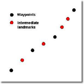
The Line of Sight MethodMock ye not; although this method is getting on for 100 years old and is increasingly redundant, it may be worth remembering should your GPS break down and you find you have left the Chinagraphs for your Dalton computer at home. Basically, pilots used to set up a route of waypoints and fly from one to the next. However, in the days before meteorlogical information services that gave wind speed and direction they had to have some way of handling drift. So, a set of intermediate landmarks were selected, and as long as these were kept visually in line then the aircraft's track would be correct. Some VFR pilots still use this method - but many seem to have forgotten it. |
 |
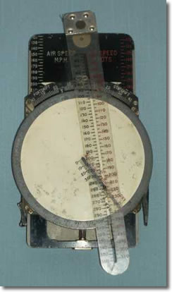 |
Course and Speed Calculator Ref. 6B/125Once meteorlogical services began to supply wind speed and direction for pilots it was possible to work out ground speed and desired compass heading on the 'triangle of forces' principle. The Course and Speed Calculator allowed the navigator to set up the wind direction and speed, the intended aircraft course and airspeed, and then read off the computed heading and resulting groundspeed. This early model was heavy and mechanically complex, but had the refinement of a small moving indicator to show drift, and also had a circular slide rule on the back. A simple example: suppose the wind is coming from the north (360 degrees) at 30 mph and you want to fly east (90 degrees) at an airspeed of 200 mph. First slide the white circle assembly along the body until the arrow on it points to 200 mph on the speed scale on the body. Now lift and swing the ruler out of the way, careful - it is delicate! Next press down on the peg and slide it all the way to the very edge of the slot. Push the peg outwards and downwards and the white disc can now be rotated so that the slot will point to any desired bearing on the compass ring. |
For this example, point the slot at 360 degrees. Now pull the peg back from the edge of the white disc and set it to the 30 mph mark in the slot. Turn the compass ring until 90 degrees is opposite the 'C' mark at the top. Now lift and swing the ruler back over the white disc so the peg is located in the ruler slot again. The peg will now indicate the computed ground speed against the mph scale on the transparent ruler (203 mph), and the drift indicator will now have moved to show the computed drift (10 degrees STBd). Most users will agree that this process is not quite as ergonomic as the later computers! |
|
RAF Navigational Computer Mk III D Ref. 6B/180The mechanically complex Calculator gave way to the more handy sliding card and rotating compass window of the Mk III of the 1940s. And being worn on the thigh it could be said to be an early wearable computer! The simplest procedure, to compute ground speed and drift, was done by rotating the window so the wind direction was opposite True Course, and moving the 'roller blind' so that the intended airspeed was under the window central dot. Suppose the wind speed was 10 knots, then a small cross was marked on the window 10 knots back from the airspeed. The window was now rotated so that the intended course was opposite True Course and, lo and behold, the small cross now shows the computed groundspeed and drift. Magic! |
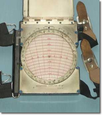 |
The speed range for this computer was from 40 to 440 mph, which was okay for the propeller era. The handy knob to move the 'roller blind' underneath the window made it easy for a pilot to do his own navigating - when it was safe to do so! There was also a circular slide rule on the top of the lid. Although simpler than the previous model, it was still relatively expensive to make. Tip: old Mk III computers very often have shrunken and cracked windows. These, like the one shown here, can be repaired using a plastic pane from a CD case. |
|
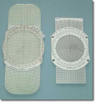 |
Computer Dead Reckoning 4A Ref. 6B/2645 and modern equivalentThe model on the left is a is model Computer Dead Reckoning 4A from the 1950s. The 'roller blind' has been replaced by a stiff plastic card which allows speeds from 80 to 800 mph. Again, there is a circular slide rule on the back. A modern civil computer is shown on the right for comparison. For some years now, navigational programs have been written for palm-top computers and so the role of the Dalton pattern computer has diminished - but it is still a handy skill to have.
|
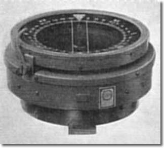
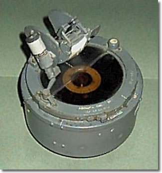
The Aperiodic CompassTo have navigated accurately in the years before electronic aids, a good compass was necessary. The RAF used high quality compasses of the aperiodic type, that is to say they settled onto a true course after a turn without any overcompensation. The reason they were so reliable was due to their sophisticated features; a strong magnetic moment, small inertia, and heavy damping. Compasses were prefixed either P for Pilot usage, or O for the Observer. This sample is a P6.
|
 |
|
|
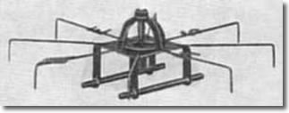
Aperiodic Compass Magnet System
The magnet system of the aperiodic compass features strong bar magnets close to the central pivot point and indicator arms that move within the damping effect of an alcohol-filled bowl. These combine to cause the magnet system to move slowly and not to overshoot. |
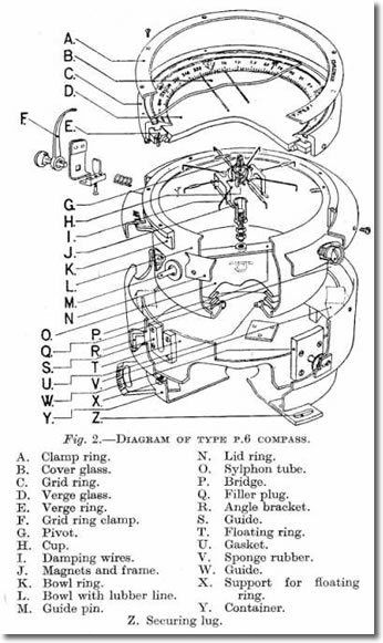
Aperiodic Compass Exploded ViewHere is an exploded view of the aperiodic compass. It is of a rather more complicated construction than most people realise. Early compasses had to have a bubble left in the damping liquid to allow for expansion in hot weather, but later ones utilised a 'Sylphon Tube Expansion Chamber', or overflow tube, which allowed the expanding damping fluid to move into it. |
 |
 |
Aperiodic Compass AdjustmentTraditionally, compasses were adjusted by placing small magnets in particular positions close to them to bring them into accurate alignment. The aperiodic compass in an aircraft was adjusted by the use of a small tool while the aircraft was jacked up in its normal flying position. |
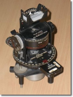
The Astro Compass Mk IIThe Astro Compass was used to take both the bearing and elevation of a celestial body, and these could then be referred to an Astronomical Almanac to establish the position of an aircraft. |
 |
 |
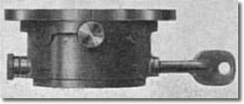
O2B Azimuth CompassThe Azimuth Compass was designed to allow navigators to obtain an accurate bearing of a geographical feature. The compass would be mounted on a fixed pole and aligned with the aircraft. By rotating a bezel on the top of the compass body, the sighting aperture would be brought into line with the feature and its bearing could then be read off the compass card through the glass prism mounted above. A small lamp housing next to the prism allowed use at night. |
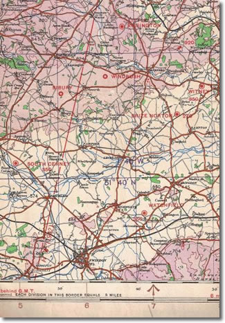
Section of WWII RAF MapWartime maps had to be of good quality to avoid accidents. Here is a section of an RAF aeronautical map of the Midlands of the UK, showing a few well-known airfield names, and a few that are now forgotten. Higher terrain on the RAF wartime maps was coloured a progressively deeper purple, which was easier to see under low cockpit lighting. Wales? Can't miss it! |
 |
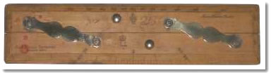 |
RAF Protractor and Parallel RuleAnother traditional tool for the chart table of the navigator. This sample has the Air Ministry stamp and is dated 1938. It is also marked "Capt. Field's Improved" & "English Make". |
Putting these two bits of information together it suggests it was made of high quality hardwood from non-renewable resources in a distant part of the Empire. |
|
How GEE worked - and how to work it! |
|
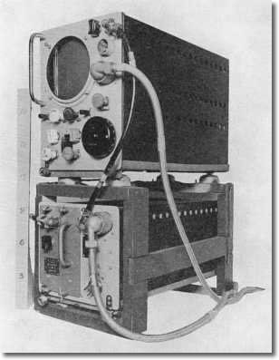
The GEE Radio Navigation System - ARI 5083The GEE Radio Navigation system was developed early in WWII. GEE (which rather boringly stood for "Grid") worked by receiving radio pulses from a number of ground stations, and by analysing the time differences between them it was possible to generate a set of co-ordinates which permitted a navigator to find the aircraft's position on a map which had a special pre-printed reference lattice overlaying the terrain. |
 |
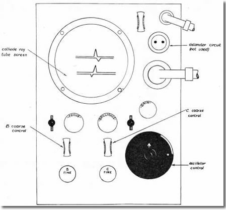 |
GEE Display and ControlsThis diagram shows the 'Indicator' - the display and set of controls of the GEE equipment. A GEE operator had to be skilled at optimising the signals displayed on the cathode ray tube (CRT) and at the the process of generating the co-ordinates, but with practice could achieve this in 30 seconds. GEE worked on VHF, i.e. line-of-sight, which meant that an aircraft above 2,000 feet could use GEE up to 250 miles from the ground stations. At 20,000 feet the range went out to 400 miles, although accuracy fell. |
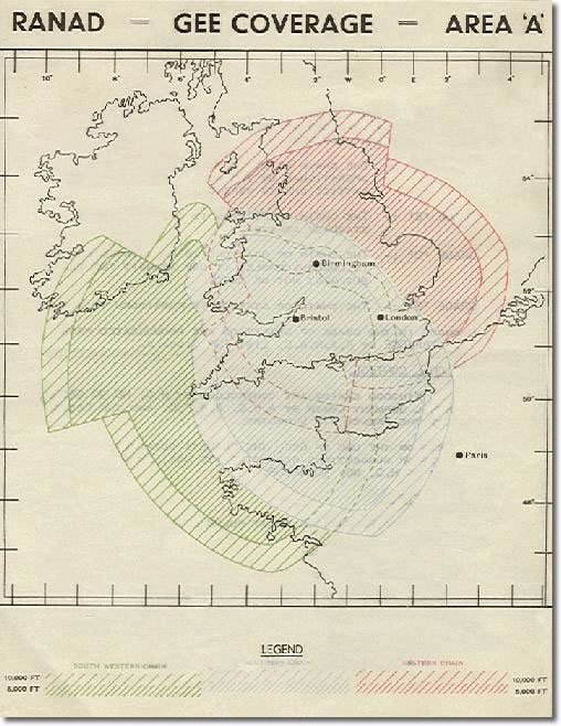
GEE Coverage Area AThe GEE system was developed as a series of chains, there being a South Western Chain, a Southern Chain, and an Eastern Chain. This diagram shows how the coverage of GEE extended as an aircraft rose from 5,000 feet to 10,000 feet. |
 |
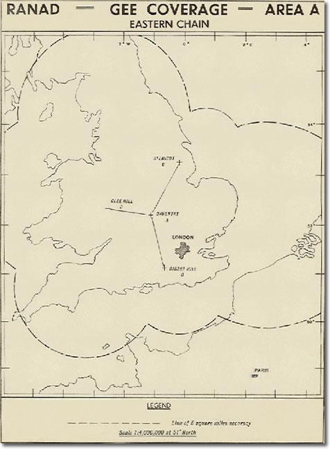 |
GEE Coverage Eastern ChainAn aircraft about to leave British airspace and head for Europe would tune into the Eastern Chain of GEE transmitter stations; the Master Station being Daventry, and the usual Slave Stations being Stenigot and Gibbet Hill. Clee Hill could also be used, but because of its position; further to the west than the other slaves, a specific time difference had to be added for it when generating the chart co-ordinates. Reception from the Master Station and one Slave could provide a position line, but an actual fix required signals from the Master and both Slaves. |
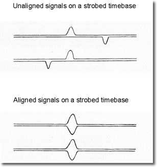
Aligning the GEE SignalsThe signals from these stations would be displayed on the CRT. Adjusting the Focus and Brilliance controls would make the signals more visible, and adjusting the Gain control until the pattern began to grow "grass" - that is to say becoming slightly fuzzy, would indicate optimum signal reception. The navigator would display a strobed timebase against which each signal could be aligned. To begin with these would not be aligned, but the navigator would use the controls to bring each signal into alignment with its reference strobe. The navigator would then go through a process which would cause the numerical co-ordinates of each signal to appear on the CRT. |
 |
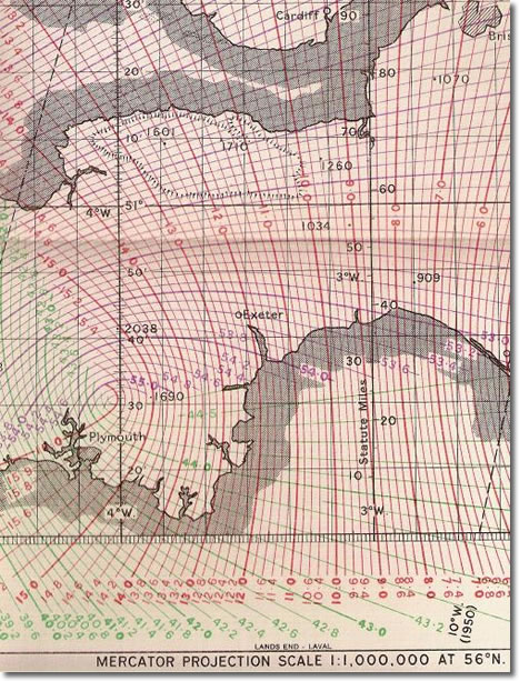 |
The GEE Lattice ChartThe co-ordinates of each station would relate to a particular set of coloured lines on the lattice chart. Slave B was Red, C was Green, and D was Purple. Accuracy depended on distance from the chain of stations, and over the UK a fix to within a few hundred yards was normal, whereas over Europe it could be a few miles. Odd weather conditions such as temperature inversions could cause signal 'ducting', in which case the range of operation could be significantly extended - and even at lower altitudes. |
Enemy jamming was often a problem. Noise jammers were often just a nuisance; but jammers that gave out bogus pulses could render GEE totally useless. The later multi-frequency GEE sets stood a better chance. But sometimes the tables were turned. Once, when a new German pulse jammer started operations, a highly switched on RAF officer reverse calculated its position and a couple of days later the jammer was bombed flat. |
|
Putting it all together, a GEE operator would fix an aircraft's position by the following means:Set left-hand tumbler switch down; right-hand tumbler switch level. Adjust Gain control until "grass" just appears on traces or signals are easily seen. With the Oscillator control, drift the signals along the traces until the single Master signal is on the extreme left of the upper trace; stop them and check any tendency to drift with the Oscillator control. With Coarse and Fine "B" controls, strobe the appropriate Slave signal on the upper trace; with Coarse and Fine "C" controls, strobe that on the lower trace. Left-hand tumbler switch to central position. With fine controls bring upper and lower Slave signals into exact alignment directly under the Master signals, check drift with Oscillator controls. Check alignment on expanded strobe time base (left-hand tumbler switch up, adjust Fine controls if necessary). Note time (this is the time of the resultant fix), and immediately depress the right-hand tumbler switch. Read off and note the correct second decimal places. Left-hand tumbler switch central, read off and note the first decimal place of top reading; left-hand tumbler switch down and note the whole number of top reading. If the "D" Slave was used, a specific value of 30 must be added. Repeat above step for lower reading, remembering to add 30 if "D" used. Enter chart with readings and plot the readings taken as position lines on or (when interpolation is necessary) between the lattice linesappropriate to the signals used(i.e., "B" on the Red lattice lines; "C" on the Green; "D" on the purple). The intersection of the position lines is the required fix. Okay, let's face it: do all that in 30 seconds and you are one hot alligator! |
© Copyright 2007 CairdPublications.com | Site Map | Contact Us |